Checkpointing Jobs#

The complexity of HPC systems can introduce unpredictable hardware or software component behavior, leading to job failures. Applying fault tolerance techniques to your HPC workflows can make your jobs more resilient to crashes, partition time limits, and hardware failures.

The Checkpointing technique#

Checkpointing is a fault tolerance technique based on the Backward Error Recovery (BER) technique, designed to overcome “fail-stop” failures (interruptions during the execution of a job).

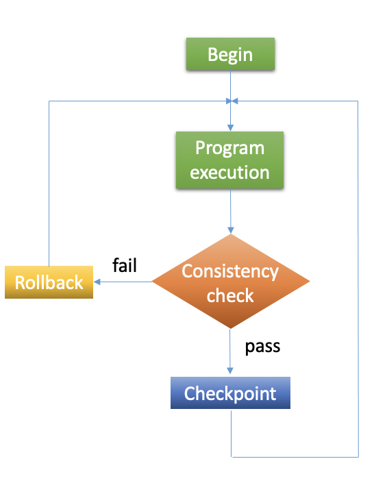
To implement checkpointing:

Use data redundancy to create checkpoint files, saving all necessary calculation state data. Checkpoint files are generally created at constant intervals during the run.
If a failure occurs, start from an error-free state, check for consistency, and restore the algorithm to the previous error-free state.

Checkpointing allows you to:

Create resilient workflows in the event of faults.
Overcome most scheduler resource time limitations.
Implement an early error detection approach by inspecting intermediate results.

Checkpointing types#

Checkpointing can be implemented at different levels of your workflow.

Application-level checkpointing is recommended for most Discovery users. You can use the checkpointing tool that is already available in your software application. For example, most software designed for HPC has a checkpointing option, and information on proper usage is often available in the software user manual.
User-level checkpointing is good if you develop your code or know the application code well enough to integrate checkpointing techniques effectively. We recommend this approach for some Discovery users with advanced proficiency and familiarity with checkpointing mechanisms.
System-level checkpointing is done on the system side, where the user saves the state of the entire process. This option is less efficient than User-level or Application-level checkpointing as it introduces a lot of redundancy.
Model-level checkpointing is suitable for saving a model’s internal state (its weights, current learning rate, etc.) so that the framework can resume the training from this point whenever desired. This is often the intent of users doing machine learning on Discovery.

Which checkpoint type should you use?#

There are several checkpointing options, depending on your software’s needs.

If your software already includes built-in checkpointing, this is often the preferred option, as it is the most optimized and efficient way to checkpoint.
Application-level checkpointing is the easiest to use, as it exists within your application. It does not require significant script changes and saves only the relevant data for your specific application.
User-level checkpointing is recommended if you are writing your code. You can use DMTCP or implement checkpointing.
ML Model-level checkpointing is specific to model training and deployment, as detailed in the ML Model-level_ section.

Note

Some packages can be used to implement checkpointing if you are developing in Python, Matlab, or R. Some examples include Python PyTorch checkpointing, TensorFlow checkpointing, MATLAB checkpointing, and R checkpointing. Additionally, many Computational Chemistry and Molecular Dynamics software packages have built-in checkpointing options (e.g., GROMACS and LAMMPS).

Implementing checkpointing can be achieved by the following:

Some save-and-load mechanisms of your calculation state.
The use of Slurm Job Arrays.

Note

To overcome partition time limits, replace your single long job with multiple shorter jobs. Then, use job arrays to set each job to run one after the other. If checkpointing is used, each job will write a checkpoint file. The following job will use the latest checkpoint file to continue from the latest state of the calculation.

Application-level checkpointing#

GROMACS checkpointing example#

The following example shows how to implement a 120-hour GROMACS job using multiple shorter jobs on the short partition. We use Slurm job arrays and the GROMACS built-in checkpointing option to implement checkpointing.

DMTCP checkpoint example#

Distributed MultiThreaded checkpointing (DMTCP) is a tool checkpoint without changing code. It works with most Linux applications, such as Python, Matlab, R, GUI, and MPI.

The program runs in the background of your program, without significant performance loss and saves the process states into checkpoint files. DMTCP is available on the cluster

module avail dmtcp
module show dmtcp
module load dmtcp/2.6.0

Since DMTCP runs in the background, it requires some changes to your shell script. See examples of checkpointing with DMTCP, which use DMTCP with a simple C++ program (scripts modified from RSE-Cambridge).

Application-level checkpointing tips#

What data should you save?

Non-temporary application data
Any application data that has been modified since the last checkpoint
Delete no longer useful checkpoints; keep only the most recent checkpoint file.

How frequently do checkpoints occur?

Too often will slow your calculation; maybe I/O is heavy and memory intensive.
Too infrequently leads to large or long rollback times.
Consider how long it takes to reach a checkpoint and restart your calculation.
In most cases, every 10–15 minutes is okay.

ML Model-level Checkpointing#

Model-level checkpointing is a technique used to periodically save the state of a machine learning (ML) model during training, enabling the training process to be resumed from the saved checkpoint in case of interruptions or premature termination. The saved state typically includes the model’s parameters, optimizer state, and essential training information (e.g., the epoch number and loss value). Model checkpoints are especially critical for long-running training jobs.

Why is Checkpointing Important in Deep Learning?#

Checkpointing is crucial in deep learning because the training process can be time-consuming and require significant computational resources. Additionally, the training process may be interrupted due to hardware or software issues. Checkpoints solve this problem by saving the model’s current state to resume where it left off.

Moreover, checkpointing also saves the best-performing model, which can be loaded for evaluation. For instance, the model’s performance can vary based on the initialization and optimization algorithms, so checkpointing provides a way to select the best model based on a performance metric.

In summary, checkpointing is essential in deep learning as it provides a way to save progress, resume training, and select the best-performing model.

TensorFlow checkpoint example#

The following example demonstrates implementing a longer ML job using the tf.keras checkpointing API and multiple shorter Slurm job arrays on the GPU partition.

The following example of the submit_tf_array.bash script:

#!/bin/bash
#SBATCH --job-name=myrun
#SBATCH --time=00:10:00
#SBATCH --partition=gpu
#SBATCH --nodes=1
#SBATCH --gres=gpu:1
#SBATCH --mem=10Gb
#SBATCH --output=%A-%a.out
#SBATCH --error=%A-%a.err
#SBATCH --array=1-10%1  #execute 10 array jobs, 1 at a time.

module load miniconda3/2020-09
source activate tf_gpu

# Define the number of steps based on the job id:
numOfSteps=$(( 500 * SLURM_ARRAY_TASK_ID ))

# Run python and save outputs to a log file corresponding to the current job task ID
python train_with_checkpoints.py $numOfSteps &> log.$SLURM_ARRAY_TASK_ID

The following checkpoint example is given in the program train_with_checkpoints.py:

checkpoint_path = "training_2/{epoch:d}.ckpt"
checkpoint_dir = os.path.dirname(checkpoint_path)
cp_callback = tf.keras.callbacks.ModelCheckpoint(
   filepath=checkpoint_path,
   verbose=1,
   save_weights_only=True,
   period=5)

See scripts, which are modified from TensorFlow Save and load models.

The Slurm option --array=1-10%1 will create 10 Slurm array tasks and run one task at a time. Note that the saved variable %A denotes the main job ID, while variable %a denotes the task ID (spanning values 1-10). Note that the output/error files are also unique to prevent different jobs from writing to the same files. The Shell variable SLURM_ARRAY_TASK_ID holds the unique task ID value and can be used within the Slurm Shell script to point to different files or variables.

To submit this job to the scheduler, use the command:

sbatch submit_tf_array.bash

PyTorch checkpoint example#

Setting up a Sample Project#

Next, we will set up a sample project to demonstrate checkpointing in PyTorch. We will create a simple neural network in PyTorch and train it on a sample dataset. The following code creates a simple neural network in PyTorch:

import torch
import torch.nn as nn
import torch.nn.functional as F

class Net(nn.Module):
    def __init__(self):
        super(Net, self).__init__()
        self.fc1 = nn.Linear(28 * 28, 128)
        self.fc2 = nn.Linear(128, 10)
    def forward(self, x):
        x = x.view(-1, 28 * 28)
        x = F.relu(self.fc1(x))
        x = self.fc2(x)
        return x

Once the neural network is defined, we can load a sample dataset and train the model. In this example, we will use the MNIST dataset in the torchvision library. The following code loads the MNIST dataset and trains the model:

import torchvision
import torchvision.transforms as transforms

transform = transforms.Compose([
    transforms.ToTensor(),
    transforms.Normalize((0.5,), (0.5,))
])

trainset = torchvision.datasets.MNIST(root='./data', train=True, download=True, transform=transform)
trainloader = torch.utils.data.DataLoader(trainset, batch_size=64, shuffle=True)
net = Net()
criterion = nn.CrossEntropyLoss()
optimizer = torch.optim.SGD(net.parameters(), lr=0.001, momentum=0.9)

for epoch in range(2):
    running_loss = 0.0
    for i, data in enumerate(trainloader, 0):
        inputs, labels = data
        optimizer.zero_grad()
        outputs = net(inputs)
        loss = criterion(outputs, labels)
        loss.backward()
        optimizer.step()
        running_loss += loss.item()
    print('Epoch %d loss: %.3f' % (epoch + 1, running_loss / len(trainloader)))

With this simple project setup, we can demonstrate checkpointing in PyTorch.

What is the model state in PyTorch?#

In PyTorch, the model state refers to the values of all the parameters, weights, and biases that define the model’s behavior. This state is stored in the model’s state_dict, a dictionary-like object that maps each layer to its parameter tensors. Additionally, the state_dict contains information about the model’s architecture and the values of the parameters learned during training.

The state_dict can be saved to a file using PyTorch’s torch.save function and loaded back into memory using torch.load. This allows for checkpointing, which saves the state of a model periodically during training so that it can be recovered in the case of a crash or interruption.

PyTorch also provides the ability to save and load the entire model, including the model’s architecture and optimizer state, using the torch.save and torch.load functions. This allows for complete checkpointing of a model’s state.

It is important to note that the state_dict only contains information about the model’s parameters, not the optimizer or other training-related information. So, to save the optimizer state, you also need to save it separately and load it back when loading the model.

In conclusion, the model state in PyTorch represents the values of all the parameters, weights, and biases that define the model’s behavior. The state is stored in the state_dict and can be saved and loaded for checkpointing purposes. By saving the model state periodically during training, you can ensure that your progress is recovered during a crash or interruption.

Saving a PyTorch Model#

Saving a Model’s `state_dict`#

To save the learnable parameters of a PyTorch model and the optimizer, we must save the model’s state_dict. We can use the torch.save function to pass the state_dict and file names as arguments. The following code demonstrates how to save the state_dict of the model:

checkpoint_path = 'checkpoint.pth'
state = {'epoch': epoch + 1,
         'state_dict': net.state_dict(),
         'optimizer': optimizer.state_dict()}
torch.save(state, checkpoint_path)

Saving the Entire Model#

In addition to saving the state_dict, we can also save the entire model, which includes the architecture, the learnable parameters, and the optimizer state. We can use the torch.save() function to save the entire model by passing the model and a filename as arguments. The following code demonstrates how to save the entire model:

model_path = 'model.pth'
torch.save(net, model_path)

Note

When saving the entire model, the custom classes used to define the model must be importable, either as a part of the project or in a separate file that can be imported.

We have seen how to save the state_dict and the entire model in PyTorch. The following section will show how to load a saved model.

Loading a PyTorch Model#

Loading a PyTorch `state_dict`#

We can use the torch.load function to load the state_dict of a saved model by passing the file name as an argument. After loading the state_dict, we can set the state_dict of the model using the model.load_state_dict method. The following code demonstrates how to load the state_dict of a saved model:

codecheckpoint = torch.load(checkpoint_path)
net.load_state_dict(checkpoint['state_dict'])
optimizer.load_state_dict(checkpoint['optimizer'])
epoch = checkpoint['epoch']

Loading the Entire PyTorch Model#

To load the entire model, use the torch.load function and pass the file name as an argument. The loaded model can then be assigned to a variable, as shown in the following code:

loaded_model = torch.load(model_path)

In PyTorch, we can load a saved model’s state_dict or the entire model. This section will cover how to resume training from a checkpoint.

Resuming Training from a Checkpoint#

To resume training from a checkpoint, we must load the model’s state_dict and the optimizer’s state (see Loading a PyTorch Model). After loading these, we can continue the training process from where it was left off. The following code demonstrates how to resume training from a checkpoint:

checkpoint = torch.load(checkpoint_path)
net.load_state_dict(checkpoint['state_dict'])
optimizer.load_state_dict(checkpoint['optimizer'])
epoch = checkpoint['epoch'] # Continue training
for epoch inrange(epoch, num_epochs): # Train the model
    # Save the checkpoint
    state = {'epoch': epoch + 1,
             'state_dict': net.state_dict(),
             'optimizer': optimizer.state_dict()
             }
torch.save(state, checkpoint_path)

This code loads the state_dict and the optimizer’s state from the checkpoint file and resumes training from the epoch value saved in the checkpoint file. After each epoch, the model’s state_dict and the optimizer’s state are saved in the checkpoint file, as described in Section III. This shows how to checkpoint PyTorch models, save and load the state_dict, save and load the entire model, and resume training from a checkpoint.

Model-level tips and tricks#

Save only the model’s State_dict#

Save only the model’s state_dict and optimizer state, allowing us to save only the information needed to resume training. Doing so reduces the checkpoint file’s size and makes it easier to load the model. So, please don’t forget to avoid unnecessary information in the checkpoint file, such as irrelevant metadata or tensors we can define during training.

Save regularly#

To prevent losing progress in case of a crash or interruption, save the checkpoint file regularly (i.e., after each epoch).

Save to multiple locations#

Save the checkpoint file to multiple locations, such as a local drive and the cloud, to ensure that the checkpoint is recovered in case of failure.

Use the latest versions of libraries#

Using the latest version of PyTorch and other relevant libraries is vital; changes in these libraries may cause compatibility issues with older checkpoints. With these best practices, you can ensure that your PyTorch models are saved efficiently and effectively and that your progress is not lost in the event of a crash or interruption.

Naming conventions#

Use a consistent naming convention for checkpoint files; include information such as the date, time, and epoch number in the file name to make tracking multiple checkpoint files easier and ensure you choose the proper checkpoint to load.

Checkpoint Validation#

Validate the checkpoint after loading it to ensure that the model’s state_dict and the optimizer’s state are correctly loaded by making a prediction using the loaded model and checking that the results are as expected.

Periodic clean-up#

Periodically, remove old checkpoint files to avoid filling up storage. This can be done by keeping only the latest checkpoint or keeping only checkpoint files from the last few epochs.

Document checkpoints#

Document the purpose of each checkpoint and what it contains: the model architecture, the training data, the hyperparameters, and the performance metrics. This will help keep track of the progress and make it easier to compare different checkpoints. With these additional best practices, you can ensure that your checkpointing process is efficient, effective, and well-organized.

Checkpointing Jobs#

The Checkpointing technique#

Checkpointing types#

Which checkpoint type should you use?#

Application-level checkpointing#

GROMACS checkpointing example#

DMTCP checkpoint example#

Application-level checkpointing tips#

ML Model-level Checkpointing#

Why is Checkpointing Important in Deep Learning?#

TensorFlow checkpoint example#

PyTorch checkpoint example#

Setting up a Sample Project#

What is the model state in PyTorch?#

Saving a PyTorch Model#

Saving a Model’s state_dict#

Saving the Entire Model#

Loading a PyTorch Model#

Loading a PyTorch state_dict#

Loading the Entire PyTorch Model#

Resuming Training from a Checkpoint#

Model-level tips and tricks#

Save only the model’s State_dict#

Save regularly#

Save to multiple locations#

Use the latest versions of libraries#

Naming conventions#

Checkpoint Validation#

Periodic clean-up#

Document checkpoints#

Saving a Model’s `state_dict`#

Loading a PyTorch `state_dict`#